As regular readers of this blog already know, Bayes factors rule! In practice, however, the calculation of Bayes factors is seriously hampered by computational difficulties. In a new paper, we revive two theorems put forth by Alan Turing and Jack Good and propose a step-by-step approach to use them as a check for the calculation of Bayes factors. According to Good, the first theorem was proposed by Turing during their work on deciphering German naval Enigma messages during World War II (for the movie lovers among you, The Imitation Game is a great way to learn how mathematics (and Bayes theorem) helped change the course of the war); subsequently, Good generalizes the first theorem by proposing his own. In this blog post, we want to give a gentle introduction to the two theorems using a simple coin toss example, and highlight the step-by-step approach that can be used to check the calculation of Bayes factors in practice.
Illustrating Turing & Good’s (Paradoxical) Theorem(s)
Imagine you flip a coin 2 times and you are interested in the number of times the coin lands heads up. It almost goes without saying that you can expect one of three possible outcomes: O1: two heads; O2: one heads and one tail; O3: two tails. Suppose we have a hypothesis H0, which says that the coin is fair, or in other words, that the probability of the coin landing heads is ½ on any one toss; the binomial distribution tells us that under H0, the probability of O1 and O3 is 1/4, and the probability of O2 is 1/2. Suppose we also have a hypothesis H1, which says that all outcomes are equally likely, that is, it assigns a probability of 1/3 to all three outcomes.
Suppose we know that H1 is true. Then the theorem proposed by Alan Turing tells us that the average Bayes factor (also called the expectation or first moment of the Bayes factor) in favor of H0 is 2 * ((1/4) / (1/3)) * 1/3 + ((1/2) / (1/3)) * 1/3 = 1. In words: The expected Bayes factor in favor of the false hypothesis is 1. This may seem paradoxical, since one would expect the average Bayes factor against the truth to be much less than 1. However, remember that the Bayes factor is not symmetric; for example, the average of a Bayes factor of 10 and 1/10 is greater than 1.
Good generalizes Turing’s theorem by linking it to higher-order (raw) moments. The theorem states that the first moment (the expected value) of the Bayes factor in favor of H1 when H1 is the true hypothesis is equal to the second moment of the Bayes factor in favor of H1 when H0 is the true hypothesis. Going back to the coin toss example, the expected value of the Bayes factor in favor of H1 when H1 is true is 2 * (1/3) / (1/4) * (1/3) + (1/3) / (1/2) * (1/3), and the second moment of the Bayes factor in favor of H1 when H0 is true is 2 * ((1/3) / (1/4))^2 * (1/4) + ((1/3) / (1/2))^2 * (1/2), both of which are approximately 1.11. Comparing the zeroth and the first moment, this theorem reduces to the first one proposed by Turing.
A Formal Check on the Bayes Factor
Using the two theorems, in the paper, we suggest the following approach to checking the calculation of Bayes factors in practice. Assume you have collected data and want to test your hypothesis using the Bayes factor, the check involves the following steps:
- Begin by defining two competing models and assigning prior distributions to their parameters.
- Use your chosen computational method to calculate the Bayes factor based on your observed data (usually using a certain software package such as JASP or a library in R).
- Decide which model you believe to be true (usually the more complex one, for the details we recommend reading the full paper) and generate synthetic data based on its prior distribution. Then compute the Bayes factor for this synthetic data. Repeat this step m times.
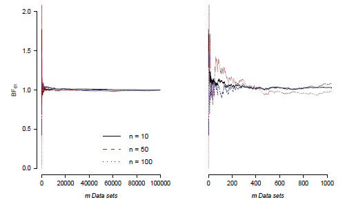
- (Theorem 1) Compute the average Bayes factor for the m synthetic data. If this average is close to 1 after many simulations, it indicates that your Bayes factor calculations are reliable.
- (Theorem 2) Repeat the simulation process, but this time assume that the other hypothesis is true. Calculate the Bayes factor for this scenario m times. Finally, compare the mean Bayes factor for the true hypothesis with the second moment of the Bayes factor for the false hypothesis. If these values are approximately the same, this provides further assurance of the accuracy of your calculations.
References
Good, I. J. (1985). Weight of evidence: A brief survey. Bayesian Statistics, 2, 249–270.
Sekulovski, N., Marsman, M., & Wagenmakers, E.-J. (2024). A Good check on the Bayes factor. https://doi.org/10.31234/osf.io/59gj8
About The Author

Nikola Sekulovski
Nikola Sekulovski is a PhD student at the University of Amsterdam.