R code for the reported analyses is available at https://osf.io/sfam7/.
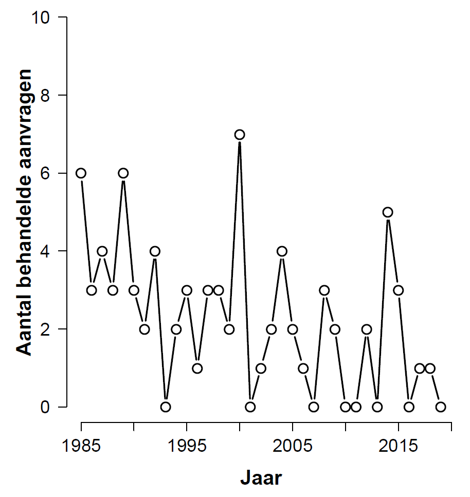
My wife Nataschja teaches labor law at Utrecht University. For one of her papers she needed to evaluate the claim that “over the past 35 years, the number of applications processed by the AAC (Advice and Arbitration Committee) has decreased”. After collecting the relevant data Nataschja asked me whether I could help her out with a statistical analysis. Before diving in, below are the raw data and the associated histogram:
Gegevens <- data.frame(
  Jaar      = seq(from=1985,to=2019),
  Aanvragen = c(6,3,4,3,6,3,2,4,0,2,3,1,3,3,2,7,0,1,2,4,2,1,
                0,3,2,0,0,2,0,5,3,0,1,1,0)
)
# NB: “Gegevens” means “Data”, “Jaar” means “Year”, and “Aanvragen” means “Applications”
NB. “Aantal behandelde aanvragen” means “number of processed applications”.
Based on a visual inspection most people would probably conclude that there has indeed been a decrease in the number of processed applications over the years, although that decrease is due mainly to the relatively high numbers of processed applications in the first five years (more on this later).
Below I will describe the analyses that I conducted without the benefit of knowing a lot about the subject area. Indeed, I also didn’t know much about the analysis itself. In experimental psychology, the methodologist feeds on a steady diet: a t-test for breakfast, a correlation for lunch, and an ANOVA for dinner, interrupted by the occasional snack of a contingency table. After some thought, I felt that this data set cried out for Poisson regression — the dependent variable are counts, and “year” is the predictor of interest. By testing whether we need the predictor “year”, we can more or less answer Nataschja’s question directly. Poisson regression has not yet been added to JASP, and this is why I am presenting R code here (the complete code is at https://osf.io/sfam7/).
Frequentist Analysis: Full Data Set
The Poisson regression model can be fit using the following R code:
pois.mod <- glm(Aanvragen ~ Jaar, data=Gegevens,
                family=poisson(link="log"))
After executing “summary(pois.mod)” we learn that the beta coefficient for the predictor “year” is -0.04051 with a standard error of 0.01170, for a z-value of -3.463 and a highly significant p-value of 0.000534. The fitted values are in “pois.mod$fitted.values” and can be shown on top of the actual data:
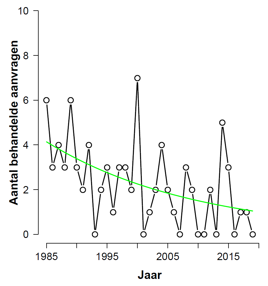
What have we learned? Well, ideally we would now be able to conclude that it is likely that the number of processed applications has decreased, or at least that the data have made it more likely than before that the number of processed applications has decreased. But the p-value does not allow such a conclusion. All that we are licensed to say is something along the lines of “the probability is low that the observed test statistic (or more extreme forms) would occur if the null hypothesis (i.e., the number of processed applications is constant over time) were true.” How disappointing.
In the preface to the first edition of Theory of Probability (1939), our Bayesian champion Harold Jeffreys stresses the fact that, ultimately, the p-value machinery cannot deliver the epistemic goods:
“Modern statisticians have developed extensive mathematical techniques, but for the most part have rejected the notion of the probability of a hypothesis, and thereby deprived themselves of any way of saying precisely what they mean when they decide between hypotheses.” (Jeffreys, 1939, p. v)
On the next page of the preface Jeffreys continues to drive home the same point:
“There is, on the whole, a very good agreement [of Bayes factors developed by Jeffreys– EJ] with the recommendations made in statistical practice; my objection to current statistical theory is not so much to the way it is used as to the fact that it limits its scope at the outset in such a way that it cannot state the questions asked, or the answers to them, within the language that it provides for itself, and must either appeal to a feature of ordinary language that it has declared to be meaningless, or else produce arguments within its own language that will not bear inspection.” (Jeffreys, 1939, p. vi)
The upshot of this is that, if we wish to know whether the data undercut the null hypothesis and support the alternative hypothesis (and what researcher would deny themselves such knowledge?) we have no choice but to embrace Bayesian inference.
Bayesian Analysis: Full Data Set
Here we use Merlise Clyde’s BAS package, which also underlies the linear regression functionality in JASP. In addition to linear regression, the BAS package also offers logistic regression and Poisson regression. The code is simple:
library(BAS)
pois.bas <- bas.glm(Aanvragen ~ Jaar, data=Gegevens,
                    family=poisson(), modelprior=uniform())
summary(pois.bas)
From the BAS output, the Bayes factor for the model including “year” versus the null model is obtained as “exp(pois.bas$logmarg[2]-pois.bas$logmarg[1])” and equals 35.4, meaning that the data are over 35 times more likely to have occurred under H1 than under H0. This outcome is qualitatively consistent with the low p-value, but provides an explicit answer to a relevant question: the data have shifted our beliefs about the relative plausibility of H1 and H0 by a factor of 35 in the direction of H1.
Analyses Without the Education Sector
An unexpected complication in the above analysis is that it contains some processed applications from the education sector, which at some point stopped being associated with the AAC. We therefore redo the above analyses, but now exclude the education sector entirely. The cleaned-up data are here:
Gegevens2 <- data.frame(
  Jaar      = seq(from=1985,to=2019),
  Aanvragen = c(6,3,3,1,4,0,1,3,0,0,1,1,2,2,2,7,0,1,1,4,2,1,
                0,3,2,0,0,2,0,5,3,0,1,1,0)
The associated histogram with the fit of the model that includes “year” is shown here:
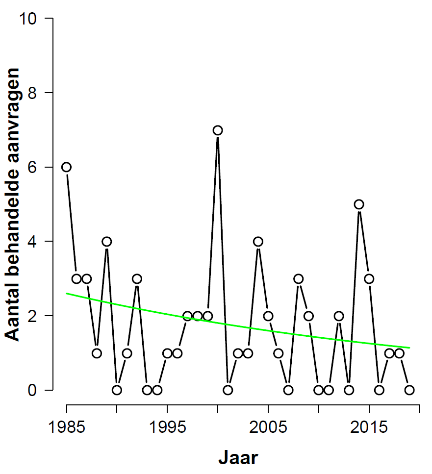
The frequentist analysis output shows that the beta coefficient for “year” is -0.02432 with a standard error of 0.01280, for a z-value of -1.900 and a p-value of 0.0574. This is not statistically significant at the god-given alpha-level of .05, but it would be significant if we conduct a one-sided test; and in this case there is a clear directional expectation. The BAS Bayes factor is 2.1 in favor of H0. Jeffreys (1939, p. 357) termed this level of evidence “not worth more than a bare comment”. The BAS parameter priors may be tinkered with, and with sufficient effort one may perhaps be able to produce a Bayes factor of, say, 2 in favor of H1. This level of evidence, however, would likewise be “not worth more than a bare comment”. Such an exercise in tinkering will demonstrate that the much-maligned prior is actually less influential than an informed (dare we say “subjective”?) decision concerning data cleaning.
In conclusion, after removal of the education section the frequentist analysis yields a somewhat ambiguous result. The Bayesian analysis suggests that the data are not diagnostic; this may be taken to mean that the data do not provide grounds to replace the null hypothesis with an alternative.
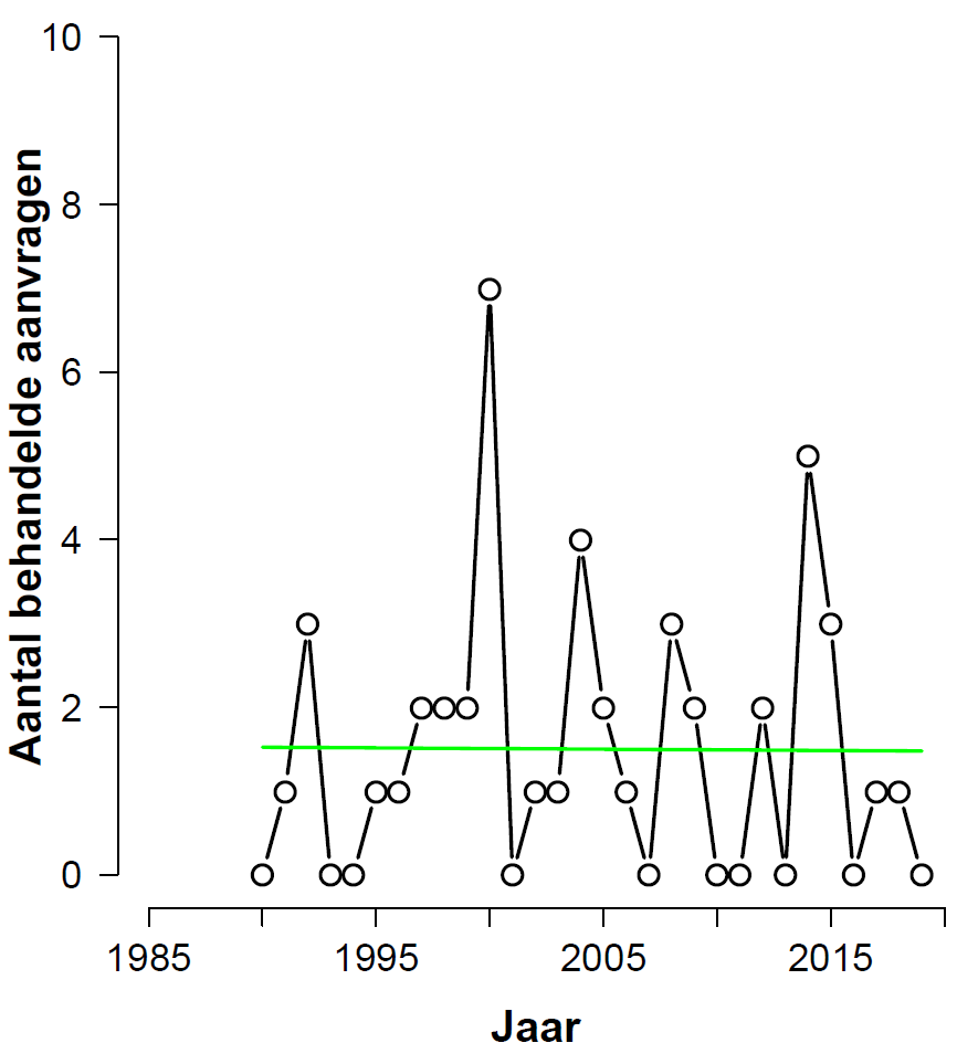
Omitting The First Five Years
The analyses discussed so far had been the ones requested by Nataschja (at least in the sense of including and excluding the education sector). Visual inspection suggested that the first few years had a large influence on the outcomes. As an exploratory analysis, and without any advance input from Nataschja, I decided to conduct the same analyses as above but now excluding the first five years.
Consider the full data set (including education), after omitting the first five years. This is the histogram with fitted values:
From the analysis output we learn that the beta-coefficient for “year” has a value of -0.03051 with a standard error of 0.01562, for a z-value of -1.953 and a p-value of 0.0508. As in the previous analysis, this is just higher than the sacred .05 level (so it will be below that level for a one-sided test). The BAS output yields a Bayes factor of 1.78 in favor of H0 — as in the previous analysis, this level of evidence is “not worth more than a bare comment”, and provides no reason to abandon the null hypothesis.
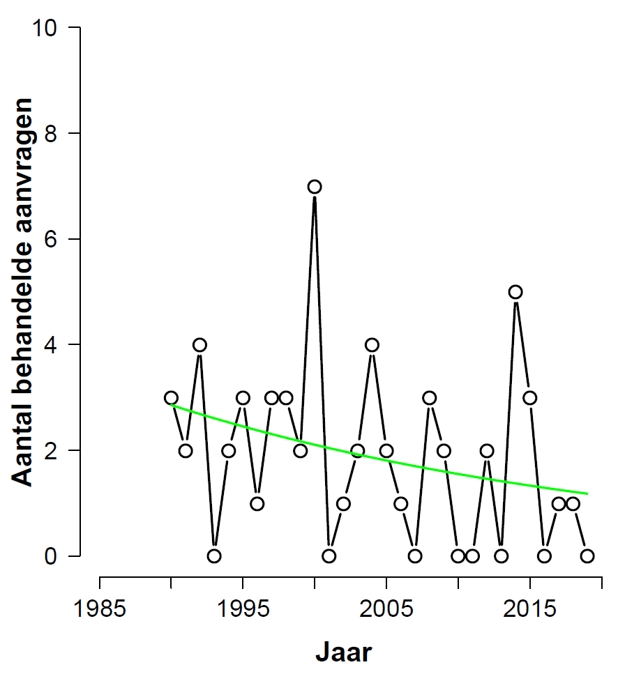
Finally we consider the clean data set (excluding education), after omitting the first five years. This is the histogram with fitted values:

From the analysis output we learn that the beta-coefficient for “year” has a value of-0.001038 with a standard error of 0.017223, for a z-value of -0.060 and a p-value of 0.952. This is nowhere near significant, but from the p-value alone there is no way of telling whether the data show absence of evidence or evidence of absence. Frequentists may feel inspired to jump through some hoops –consider confidence intervals, conduct equivalence tests, contemplate power– but ultimately these prosthetics fail to provide an answer to the question of the degree to which the data support H0 versus H1. To address this question we apply the BAS package once more and find a Bayes factor of 11.4 in favor of H0: evidence of absence, not absence of evidence.
Conclusion
We used Poisson regression to answer the claim that “over the past 35 years, the number of applications processed by the AAC (Advice and Arbitration Committee) has decreased”. The first analyses (both frequentist and Bayesian) supported this claim, although only the Bayesian analysis was able to address it directly. However, it then turned out that the original data were contaminated; after clean-up, the two-sided p-value was just higher than the holy threshold of .05; the Bayes factor was not diagnostic, suggesting that there is no need to abandon the null hypothesis. An exploratory analysis supported the visual impression that the first five years featured a relatively high number of processed applications. For the cleaned data, omitting the first five years eliminated any trace of an effect. As an aside, Nataschja believes that the “first-five-year effect” is not unexpected, as a 1989 change in law saw the introduction of an “overeenstemmingsvereiste” (requirement of agreement) which leveled the playing field in labor law negotiations and may have lessened the need for the AAC. Of course, testing this explanation rigorously would require a more subtle approach, such as including the first five years as a separate predictor.
References
Clyde, M. (2016). BAS: Bayesian Adaptive Sampling for Bayesian model averaging. R package version 1.4.1.
Hummel, N. (2020). Het ‘vergeten’ derde lid van artikel 6 ESH. Manuscript submitted for publication.
Jeffreys, H. (1939). Theory of Probability. Oxford: Oxford University Press.
About The Author

Eric-Jan Wagenmakers
Eric-Jan (EJ) Wagenmakers is professor at the Psychological Methods Group at the University of Amsterdam.