In a previous blog post, we proposed the following test of your Bayesian intuition:

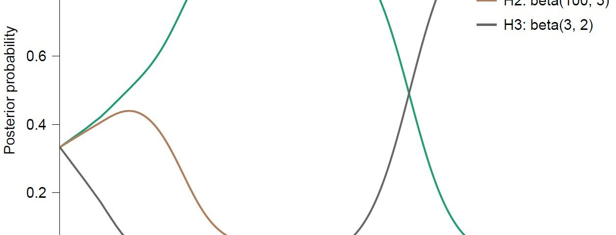
Three friends –Alex, Bart, and Cedric– each assign their own prior distribution to a binomial chance parameter θ. Let’s say that θ is the chance that Harriet bakes a vegan pancake rather than a bacon pancake. Alex assigns θ a beta(300,3) prior distribution, indicating a strong belief in high values of θ (i.e., Alex predicts that almost all of Harriet’s pancakes will be vegan). Bart assigns θ a beta(100,3) prior distribution, also indicating a strong belief in high values of θ (but less strong than that of Alex). Finally, Cedric assigns θ a beta(3,2) prior distribution, reflecting a very weak belief in high values of θ (i.e., Cedric has little information and refuses to issue precise predictions). For your convenience, the prior distributions are visualized below.

After specifying the prior distributions, Harriet starts baking pancakes. All of her pancakes turn out to be vegan. Harriet is quite industrious and who does not like a tasty pancake? Consequently, the unbroken sequence of vegan pancakes soon runs into thousands, hundreds of thousands, and then millions. The question is this: which of the three friends best predicted the observed unbroken sequence of vegan pancakes? 

The Answer

Most people’s intuition would suggest that Alex does best, followed by Bart, and then Cedric. After all –in line with the explanation by ChatGPT– Cedric’s beta distribution reflects a lack of commitment to any particular value of θ, whereas the beta distribution from Alex (and, to a slightly lesser extent, from Bart) has most of its mass near θ=1, which is the data-generating process. This intuition is correct, but only at the start of the pancake baking process. As Harriet produces more and more pancakes, Cedric gradually but inevitably starts to outpredict Alex and Bart. Here is a plot from the LearnBayes module in JASP:

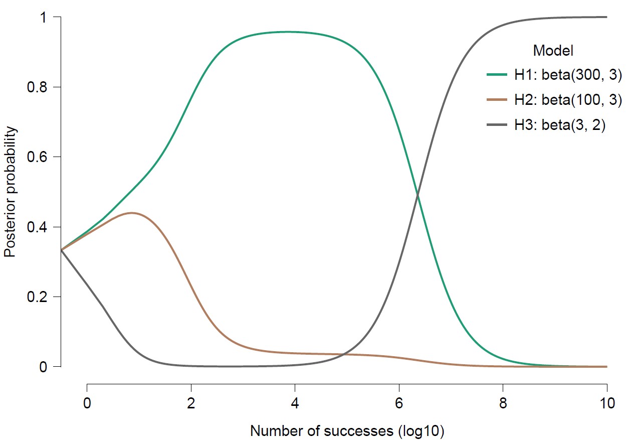
This is a surprising result. One attempt at explaining it runs as follows. As the number of vegan pancakes accumulate, the first parameter of the beta distribution grows very large, for all three forecasters. The second parameter, however, is never updated. Moreover, that second parameter determines the tail behavior of the posterior distribution near θ=1. This is even more important because all forecasters use a misspecified model — that is, all forecasters deny the truth (i.e., θ=1) with absolute certainty, as the second parameter of the beta distribution is larger than 1. Consequently, the second parameter of the beta distribution determines the asymptotic relative predictive performance.

As another demonstration, consider the predictive performance of Amy, who assigns θ a beta(2,2) prior distribution, versus that of Jane, who assigns θ a beta(2,2.2) prior distribution. These two distributions are highly similar. However, the second parameter is a fraction smaller for Amy than it is for Jane, and this implies that Amy will outperform Jane — and that Amy’s predictive advantage will grow without bound as the number of vegan pancakes accumulate. To demonstrate, here is another plot from the LearnBayes module in JASP:

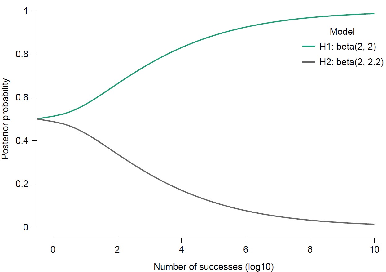
This is a vivid demonstration of how minute differences in the prior distribution can cause infinitely large differences in relative predictive success. It is important to note that this pattern is quite different if the true value of θ falls in between 0 and 1; in these cases, the forecasters would not use misspecified models, and the relative predictive performance would approach a bound that equals the ratio of prior ordinates evaluated at the data-generating value of θ (e.g., Ly & Wagenmakers, 2023, and references therein). A more mathematical analysis will be presented in the next update of the free course book  (in the appendix chapter “Statistical Analysis of the Binomial Distribution”). 

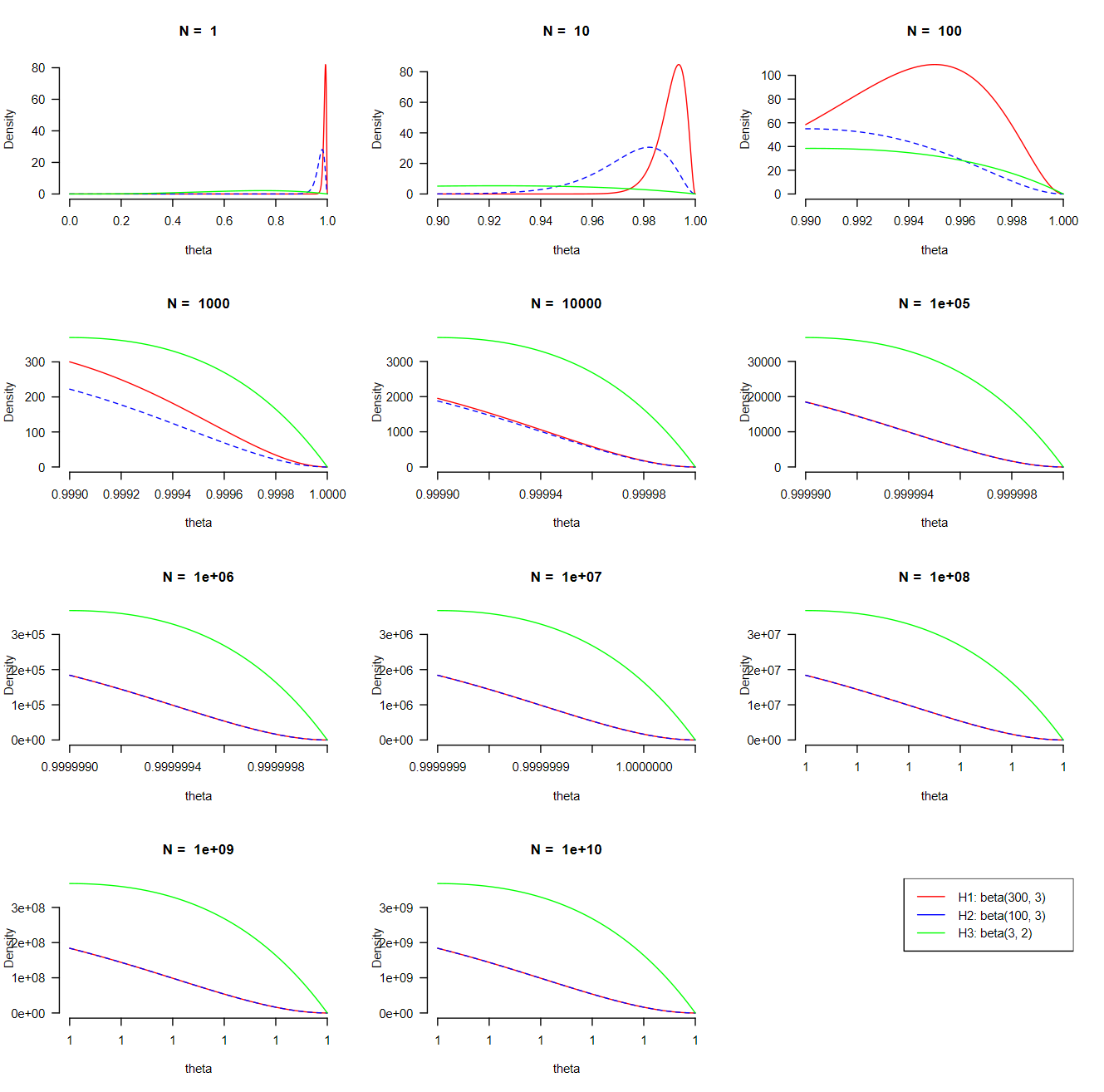
Now Erik-Jan van Kesteren, a former JASP team member, may have had the right intuition. On Mastodon, he asked “show us the density plots from 0.99-1.00 ;-)”. Well, Erik-Jan, see the plot below. Every new panel has an order of magnitude more observations, and zooms into the area near θ by the same fraction. As the data accumulate, the tails for the beta posteriors from Alex and Bart start to coincide (“the data overwhelm the prior”); however, the posterior from Cedric is consistently closer to θ=1 after about 1000 pancakes. It is interesting that the tails of the three distributions retain almost the same shape (with the right scaling applied).    

References

Ly, A., & Wagenmakers, E.-J. (2022). Bayes factors for peri-null hypotheses. TEST, 31, 1121-1142.

Authors

EJ Wagenmakers and František Bartoš.