This post is a synopsis of Boehm U, Evans N J, Gronau D., Matzke D, Wagenmakers E.-J., & Heathcote A J. (2021). Computing and using inclusion Bayes factors for mixed fixed and random effect diffusion decision models. Preprint available at https://psyarxiv.com/45t2w
Abstract
Cognitive models provide a substantively meaningful quantitative description of latent cognitive processes. The quantitative formulation of these models supports cumulative theory building and enables strong empirical tests. However, the non-linearity of these models and pervasive correlations among model parameters pose special challenges when applying cognitive models to data. Firstly, estimating cognitive models typically requires large hierarchical data sets that need to be accommodated by an appropriate statistical structure within the model. Secondly, statistical inference needs to appropriately account for model uncertainty to avoid overconfidence and biased parameter estimates. In the present work we show how these challenges can be addressed through a combination of Bayesian hierarchical modeling and Bayesian model averaging. To illustrate these techniques, we apply the popular diffusion decision model to data from a collaborative selective influence study.
Highlights
Cognitive models provide many advantages over a-theoretical statistical and
psychometric measurement models of psychological data. Moving beyond the merely
descriptive, their parameter estimates support a theoretically motivated account of latent
psychological processes that leverages the cumulative results of previous research (Farrell & Lewandowsky, 2018).” While cognitive models convey considerable merit for cumulative theory building, “estimation and inference for [these] models is difficult because they are usually highly non-linear, [and ‘sloppy’, a term used in mathematical biology for models with highly correlated parameters (Gutenkunst et al., 2007)].
As a first challenge, cognitive models need to appropriately account for hierarchical data structures. ‘Sloppiness’ and the pervasive non-linearity mean that successfully fitting cognitive models like the DDM to individual participants’ data often requires each participant to perform a large number of trials (Lerche et al., 2016). […] Unfortunately, simple techniques that average small amounts of data from each member of a large group of participants to compensate for the small number of trials per participant can produce misleading results due to non-linearity (Heathcote et al., 2000). This limits the effectiveness of cognitive modeling in settings such as clinical psychology and neuroscience where it is often not practical to obtain many trials from each participant. […] Mixed or hierarchical models, which provide simultaneous estimates for a group of participants, provide a potential solution to [this challenge]. They avoid the problems associated with simple averaging while improving estimation efficiency by shrinking individual participant estimates toward the central tendency of the group (Rouder et al., 2003).
As a second challenge, inference for cognitive models needs to appropriately account for model uncertainty. Many applications of cognitive models aim to identify relationships between cognitive processes that are represented by model parameters and a manifest variable, such as an experimental manipulation or individual differences in some observable property. To this end, researchers specify a set of candidate models, each of which allows a subset of the model parameters to covary with the manifest variable while constraining all other model parameters to be equal across levels of the manifest variable. Inference can then proceed by selecting the model that best accounts for the data. Bayes factors are a classical method for model selection that appropriately penalizes for model complexity (Kass & Raftery, 1995). However, it may be undesirable to base inference on a single model due to model uncertainty. Because only finite amounts of data are available, the correct model can never be known with certainty. […] Fortunately, inference can instead be based on a weighted average of the complete set of candidate models that takes both model complexity and model uncertainty into account (Hoeting et al., 1999).
[In this paper,] we implement the [Bayesian] framework for the DDM and test its application to Dutilh et al.’s (2019) data from a blinded collaborative study that challenged analysts to identify selective influences of a range of experimental manipulations on evidence-accumulation processes. We assess the performance of our estimation and inference methods with these data and with synthetic data generated from parameters estimated from the empirical data.
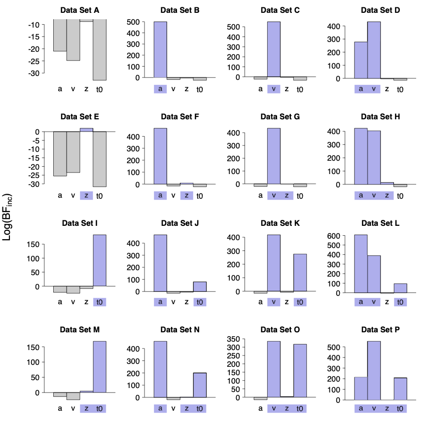
Figure 6 shows the log-inclusion Bayes factors for the four core DDM parameters for the 16 simulated data sets. [Blue bars indicate parameters that were varied between conditions in the data generating model. The Bayes factors] support the inclusion of all of the parameters that differed between conditions in the generating model. However, in the data sets where the z parameter was manipulated (data sets E – H and M – P), the inclusion Bayes factors only provide weak support. The evidence against the inclusion of parameters that were not manipulated is generally much weaker than the evidence for the inclusion of parameters that were manipulated, which is a general property of Bayes factors where the point of test falls inside the prior distribution (see Jeffreys, 1939). However, with the exception of z, the evidence was usually still overwhelming (i.e., ≤ 20), which can be best seen with data set A because of the smaller range of values displayed.

Figure 6
Log-inclusion Bayes factors for 16 simulated data sets. Blue bars indicate parameters that were varied between conditions in the data generating model.
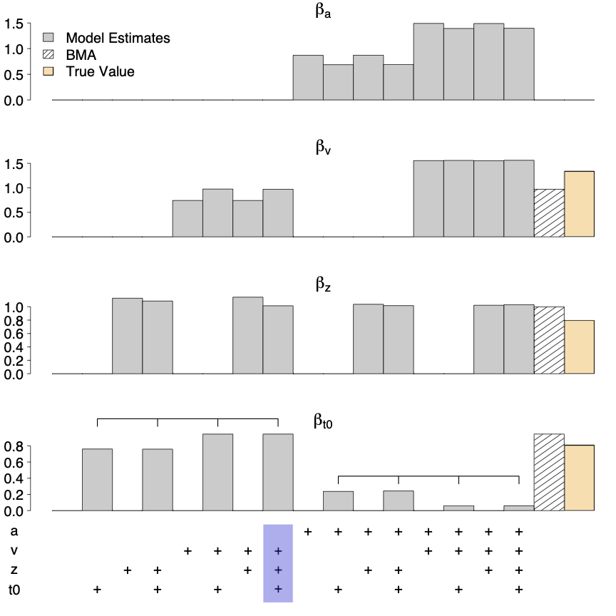
We illustrate the utility of BMA parameter estimates in Figure 7. It shows effect estimates (β) for the the four main DDM parameters produced by the 16 models fit to data set O, where true effects were present for all but a. Gray bars show the individual model effect estimates, the shaded bar shows the model-averaged estimate, and the orange bar shows the generating value (for a the latter two are zero). As can be seen, parameter estimates varied considerably between the individual models. For instance, models that allowed non-decision time but not boundary separation to vary between conditions (indicated by the leftmost brace) produced non-decision time effect estimates close to the true effect. In contrast, models that allowed both non-decision time and boundary separation to vary between conditions (indicated by the rightmost brace), severely underestimated the non-decision time condition effect. Hence, if researchers base parameter estimation on a single model, selecting the wrong model can considerably bias parameter estimates. In contrast, the model-averaged parameter estimates (shaded bars) are close to the true value for all four parameters.

Figure 7
Estimates of the condition effects (βθ) on the core DDM parameters for simulated data set O. The blue bar at the bottom indicates the generating model. The BMA estimate for βa is numerically indistinguishable from 0 and is therefore not visible.
References
Dutilh, G., Annis, J., Brown, S. D., Cassey, P., Evans, N. J., . . . Donkin, C. (2019). The quality of response time data inference: A blinded, collaborative assessment of the validity of cognitive models. Psychonomic Bulletin & Review, 26, 1051–1069. https://doi.org/10.3758/s13423-017-1417-2
Farrell, S., & Lewandowsky, S. (2018). Computational modeling of cognition and behavior. Cambridge University Press. https://doi.org/10.1017/CBO9781316272503
Gutenkunst, R. N., Waterfall, J. J., Casey, F. P., Brown, K. S., Myers, C. R., & Sethna, J. P. (2007). Universally sloppy parameter sensitivities in systems biology models. PLoS Computational Biology, 3 (10), e189. https://doi.org/10.1371/journal.pcbi.0030189
Heathcote, A., Brown, S., & Mewhort, D. J. K. (2000). The power law repealed: The case for an exponential law of practice. Psychonomic Bulletin & Review, 7 (2), 185–207. https://doi.org/10.3758/BF03212979
Hoeting, J. A., Madigan, D., Raftery, A. E., & Volinsky, C. T. (1999). Bayesian model averaging: A tutorial. Statistical Science, 14 (4), 382–417. https://www.jstor.org/stable/2676803
Jeffreys, H. (1939). Theory of probability (1st ed.). Oxford University Press.
Kass, R. E., & Raftery, A. E. (1995). Bayes factors. Journal of the American Statistical Association, 90 (430), 773–795. https://doi.org/10.2307/2291091
Lerche, V., Voss, A., & Nagler, M. (2017). How many trials are required for robust parameter estimation in diffusion modeling? A comparison of different estimation algorithms. Behavior Research Methods, 49 (2), 513–537. https://doi.org/10.3758/s13428-016-0740-2
Rouder, J. N., Sun, D., Speckman, P. L., Lu, J., & Zhou, D. (2003). A hierarchical Bayesian statistical framework for response time distributions. Psychometrika, 68 (4), 589–606. https://doi.org/10.1007/BF02295614
About The Author

Udo Boehm
Udo Boehm is postdoc at the Psychological Methods Group at the University of Amsterdam.


