How to Memorize Bayes’ Rule

September 06 - 2024

Bayes’ rule dictates how new data $y$ update the credibility of competing accounts of the world $\theta$ . An immediate consequence of the definition of conditional probability, Bayes’ rule is usually presented as follows:

$\displaystyle p(A \mid B) = \frac{p(A) \times p(B \mid A)}{p(B)} .$

The way I mentally check this equation is to take the denominator of the expression on the right-hand side, $p(B)$ , and multiply it with the left side of the equation, so we have $p(A \,|\, B) \times p(B)$ , which equals $p(A,B)$ by the definition of conditional probability. This is the same as the numerator on the right-hand side of the equation, namely $p(A) \times p(B \,|\, A) = p(B,A) = p(A,B)$ .

Below I will present two ways in which students might memorize Bayes’ rule without directly using the law of conditional probability. This will become easier when we give meaning to the abstract symbols $A$ and $B$ . In the following we replace $A$ with $\theta$ (indexing rival accounts of the world) and we replace $B$ with $y$ (observed data), so we are trying to memorize or reconstruct this version of Bayes’ rule:

$\displaystyle p(\theta \mid y) = \frac{p(\theta) \times p(y \mid \theta)}{p(y)} .$

This can be rewritten and interpreted as follows:

$\displaystyle \underbrace{ p(\theta \mid y)}_{\substack{\text{Posterior for }\theta:\\ \text{new beliefs} }} \,\,\,\, = \underbrace{ p(\theta)}_{\substack{\text{Prior for }\theta:\\ \text{old beliefs} }} \,\, \times \,\,\, \underbrace{\frac{p(y \mid \theta)}{p(y)}}_{\substack{\text{Relative predictive}\\ \text{adequacy for }\theta } }.$

Method 1: Surprise lost is credibility gained

We may take the above equation and divide both sides by $p(\theta)$ in order to obtain the following expression (cf. Rouder & Morey, 2019; see this blogpost for more detail):

$\displaystyle \frac{p(\theta \mid y)}{p(\theta)} = \frac{p(y \mid \theta)}{p(y)}.$

The left-hand side of the equation shows the change in credibility brought about by taking into account the observed data $y$ ; the right-hand side shows the relative predictive adequacy for $\theta$ , that is, the change in surprise resulting from conditioning on $\theta$ . When conditioning on a particular hypothesis $\theta$ makes the data less surprising, this hypothesis gains credibility: surprise lost is credibility gained. The aspect that makes this equation easy to recall is that the left-hand side is just the same as the right-hand side, but with $y$ and $\theta$ switched.

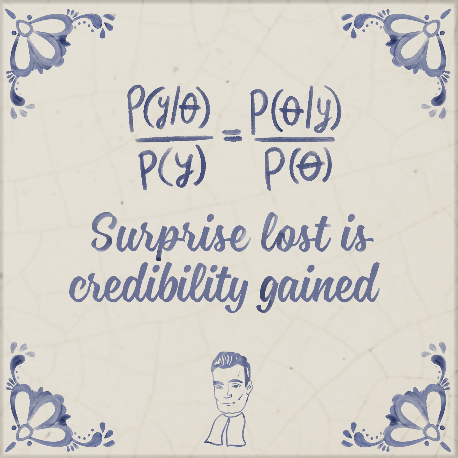
Tile designed by Viktor Beekman, CC-BY.

Method 2: Conceptual reconstruction

The second method to reproduce Bayes’ rule is based on a number of insights. We start by writing down $p(\theta \mid y)$ , because this is what we want to know: our knowledge of $\theta$ after observing data $y$ . We know that this has to involve a change from our knowledge before observing data $y$ , so we are ready to write $p(\theta \mid y) = p(\theta) \times U$ , where $U$ is the updating factor. Now this updating factor consists of two components, and these can be remembered easily from the following considerations. First, we know that $U$ needs to involve a division by $y$ . This is actually right there in the equation: when we write $p(\theta \mid y)$ , the verical stroke is inspired by the slanted division sign (see the post “The man who rewrote conditional probability” for details). Second, in the numerator of this division there needs to be our final ingredient, $p(y \mid \theta)$ . The reason why this has to be there is because otherwise Bayes’ rule would not achieve its actual objective, which is to infer something about the possible causes $\theta$ based on the observed data $y$ (i.e., $p(\theta \mid y)$ ) based partly on the inverse information: the predictive adequacy for observed data $y$ based on assumed causes $\theta$ (i.e., $p(y \mid \theta)$ ).

References

Rouder, J. N., & Morey, R. D. (2019). Teaching Bayes’ theorem: Strength of evidence as predictive accuracy. The American Statistician, 73, 186-190.