Misconception: The Relative Belief Ratio Equals the Marginal Likelihood

March 05 - 2020

The Misconception

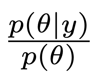
The relative belief ratio (e.g., Evans 2015, Horwich 1982/2016) equals the marginal likelihood.

The Correction

The relative belief ratio is proportional to the marginal likelihood. Dividing two marginal likelihoods (i.e., computing a Bayes factor) cancels the constant of proportionality, such that the Bayes factor equals the ratio of two complementary relative belief ratios (Evans 2015, p.109, proposition 4.3.1).

The Explanation

In the highly recommended book Measuring statistical evidence using relative belief, Evans (2015) defines evidence as follows (see also Carnap 1950, pp. 326-333; Horwich 1982/2016, p. 48; Keynes 1921, p. 170):

$\begin{equation} \text{Evidence for } \theta = \frac{p(\theta \mid \text{data})}{p(\theta)}, \end{equation}$

where $\theta$ represents a parameter (or, more generally, a model, a hypothesis, a claim, or a proposition). In other words, data provide evidence for a claim $\theta$ to the extent that they make $\theta$ more likely than it was before. This is a sensible axiom; who would be willing to argue that data provide evidence for a claim when they make that claim less plausible than it was before?

Evans formulates the Principle of Evidence as follows: “If $P(A | C) > P(A)$ , then there is evidence in favor of $A$ being true because the belief in $A$ has increased. If $P(A | C) < P(A)$ , then there is evidence against $A$ being true because the belief in $A$ has decreased. If $P(A | C) = P(A)$ , then there is neither evidence in favor of $A$ nor against $A$ because the belief in $A$ has not changed.” (Evans 2015, p. 96). For concreteness, consider the scenario where we entertain only two models, $\mathcal{M}_1$ and $\mathcal{M}_2$ . The relative belief ratio (RB) for $\mathcal{M}_1$ is

$\begin{equation} \text{RB}(\mathcal{M}_1 \mid \text{data}) = \frac{p(\mathcal{M}_1 \mid \text{data})}{p(\mathcal{M}_1)}, \end{equation}$

and the relative belief ratio for $\mathcal{M}_2$ is

$\begin{equation} \text{RB}(\mathcal{M}_2 \mid \text{data}) = \frac{p(\mathcal{M}_2 \mid \text{data})}{p(\mathcal{M}_2)} = \frac{1 - p(\mathcal{M}_1 \mid \text{data})}{1 - p(\mathcal{M}_1)}. \end{equation}$

Here we examine how the RB is related to the marginal likelihood and the Bayes factor. The Bayes factor quantifies the extent to which the data warrant an update from prior to posterior model odds:

$\underbrace{ \frac{p(\mathcal{M}_1 \mid \text{data})}{p(\mathcal{M}_2 \mid \text{data})}}_{\text{Posterior odds}} = \underbrace{ \frac{p(\mathcal{M}_1)}{p(\mathcal{M}_2)}}_{\text{Prior odds}} \,\, \times \,\,\,\, \underbrace{ \frac{p(\text{data} \mid \mathcal{M}_1)}{p(\text{data} \mid \mathcal{M}_2)}}_{\text{Bayes factor}}.$

The above equation shows that the Bayes factor is also the ratio of two marginal likelihoods, that is, the relative predictive adequacy for the observed data under the rival models. When the Bayes factor $\text{BF}_{ }$ is larger than 1, $\mathcal{M}_1$ outpredicts $\mathcal{M}_2$ ; when $\text{BF}_{ }$ is smaller than 1, $\mathcal{M}_2$ outpredicts $\mathcal{M}_1$ ; and when $\text{BF}_{12}$ equals 1, $\mathcal{M}_1$ and $\mathcal{M}_2$ predict the data equally well. To see the relation with the RB, we may rearrange the above equation as follows (Evans 2015, p. 109, proposition 4.3.1):

$\underbrace{ \frac{p(\text{data} \mid \mathcal{M}_1)}{p(\text{data} \mid \mathcal{M}_2)} }_{\text{BF}_{12}} = \underbrace{ \frac{p(\mathcal{M}_1 \mid \text{data})}{p(\mathcal{M}_1)} }_{\text{RB}(\mathcal{M}_1 \mid \text{data})} \Big/ \,\, \underbrace{ \frac{p(\mathcal{M}_2 \mid \text{data})}{p(\mathcal{M}_2)} }_{\text{RB}(\mathcal{M}_2 \mid \text{data})}.$ (1)

In words, the Bayes factor is the ratio between the two relative belief ratios for the competing models. When only two models are in play, the probabilities involving $\mathcal{M}_2$ can be rewritten as the complement of $\mathcal{M}_1$ , and the Bayes factor may be interpreted as a scaling operation on the relative belief ratio.

But now we have

$\underbrace{ \frac{p(\text{data} \mid \mathcal{M}_1)}{p(\text{data} \mid \mathcal{M}_2)} }_{\text{BF}_{12}} = \frac{\text{RB}(\mathcal{M}_1 \mid \text{data})}{\text{RB}(\mathcal{M}_2 \mid \text{data})},$

and this invites the interpretation that the marginal likelihood under model $\mathcal{M}_\cdot$ , that is, $p(\text{data} | \mathcal{M}_\cdot)$ , equals the relative belief ratio for that model, $\text{RB}(\mathcal{M}_\cdot | \text{data})$ . That this interpretation is false is evident from a simple counterexample. Consider two data sets, one large and one small, that yield the exact same $\text{BF}_{12}$ ; these data sets necessitate the same adjustment in beliefs, and therefore produce the same relative belief ratios $\text{RB}(\mathcal{M}_1 |\text{data})$ and $\text{RB}(\mathcal{M}_2 | \text{data})$ . However, the marginal likelihood for the large data set will usually be much lower than that of the small data set. Thus, we have that $p(\text{data} | \mathcal{M}_\cdot) \propto \text{RM}(\mathcal{M}_\cdot | \text{data})$ , where the constant of proportionality is the same for $\mathcal{M}_1$ and $\mathcal{M}_2$ .

Remark 1

When the two components of the relative belief ratio are known, the Bayes factor is determined as per Equation 1; However, when the two components of the Bayes factor are known (i.e., the marginal likelihoods of the two rival models), this does not determine the separate relative belief ratios; the relative belief ratios depend on the prior model probabilities, whereas the Bayes factor considers only the models’ relative predictive performance.

Remark 2

The Bayes factor accords with Evans’ Principle of Evidence. Suppose that $\text{RB}(\mathcal{M}_1 | \text{data}) = 1$ ; then $p(\mathcal{M}_1 | \text{data}) = p(\mathcal{M}_1)$ , and both RBs in Equation 1 evaluate to 1 such that $\text{BF}_{12} = 1$ also. Further, suppose that $\text{RB}(\mathcal{M}_1 | \text{data}) > 1$ ; then $p(\mathcal{M}_1 | \text{data}) > p(\mathcal{M}_1)$ , and consequently $[1 - p(\mathcal{M}_1 | \text{data})] / [1 - p(\mathcal{M}_1)] < 1$ , so $\text{BF}_{12} > 1$ .

Remark 3

Evans (2015, p. 109, proposition 4.3.1) also provides the following identity:

$\text{RB}(\mathcal{M}_1 \mid \text{data}) = \frac{\text{BF}_{12}}{1 - p(\mathcal{M}_1) + p(\mathcal{M}_1) \, \text{BF}_{12}}.$ (2)

Using this identity, it is straightforward to demonstrate that the relative belief ratio and the Bayes factor may order evidence differently. For instance, consider two scenarios. In scenario A we have $\text{BF}_{12} = 4$ , and in scenario B we have $\text{BF}_{12} = 2$ . In both scenarios model $\mathcal{M}_1$ outpredicts $\mathcal{M}_2$ , but the difference in predictive performance is largest in scenario A. From the perspective of Bayes factors, scenario A yields stronger evidence in favor of $\mathcal{M}_1$ than does scenario B. Consider now that in scenario A, we have $p(\mathcal{M}_1) = .90$ , that is, $\mathcal{M}_1$ is more plausible a priori than $\mathcal{M}_2$ . As per Equation 2, the associated relative belief ratio is $\nicefrac{40}{37} \approx 1.08$ . In scenario B, assume we have $p(\mathcal{M}_1) = .10$ , that is, $\mathcal{M}_1$ is less plausible a priori than $\mathcal{M}_2$ . The associated relative belief ratio is $20/11 \approx 1.82$ . From the perspective of relative belief ratios, scenario B yields stronger evidence for $\mathcal{M}_1$ than does scenario A — a reversal from the ordering given by the Bayes factor!

Remark 4

Assume $p(\mathcal{M}_1) = .50$ . If $p(\mathcal{M}_1 | \text{data}) = .99$ , then $\text{RB}(\mathcal{M}_1 | \text{data}) = .99/.50 = 1.98$ ; if $p(\mathcal{M}_1 | \text{data}) = .999$ , then $\text{RB}(\mathcal{M}_1 | \text{data}) = .999/.50 = 1.998$ ; finally, if $p(\mathcal{M}_1 | \text{data}) = .9999$ , then $\text{RB}(\mathcal{M}_1 | \text{data}) = .9999/.50 = 1.9998$ . These three relative belief ratios ( $1.98$ , $1.998$ , $1.9998$ ) are numerically close, and may suggest that the evidence is of similar strength. In contrast, the respective Bayes factors are $(.99/.50) / (.01/.50) = 99$ , $(.999/.50) / (.001/.50) = 999$ , and $(.9999/.50) / (.0001/.50) = 9999$ — each one differs from its predecessor by an order of magnitude. More dramatically still, suppose $\mathcal{M}_1$ holds ‘not all zombies are hungry’ whereas $\mathcal{M}_2$ holds ‘all zombies are hungry’. A satiated zombie is observed. With $p(\mathcal{M}_1) = p(\mathcal{M}_2) = \frac{1}{2}$ , the relative belief ratio $RB(\mathcal{M}_1 | \text{at least one satiated zombie}) = 1/(\frac{1}{2}) = 2$ . The Bayes factor in favor of $\mathcal{M}_1$ , in contrast, is infinity — the observation that occurred was deemed impossible under $\mathcal{M}_2$ , so this model is `irrevocably exploded’ by the data (Polya, 1954).

Remark 5

The Bayes factor assesses evidence by quantifying relative predictive performance, which depends solely on the marginal likelihood and is unaffected by the prior model probabilities. In contrast, the relative belief ratio involves the prior model probability as a crucial component.

Remark 6

There is a special case where the relative belief ratio does correspond to a Bayes factor. This case arises when there exists a single overarching `encompassing’ model, $\mathcal{H}_e$ , and it is of interest to quantify the degree to which the data provide support for a restriction of that model’s parameter space.

For concreteness, let $\mathcal{M}_e$ denote the encompassing model under which the prior distribution for a binomial parameter $\theta$ is assigned a uniform distribution: $\theta | \mathcal{M}_e \sim \text{beta}(1,1)$ . We consider two complementary restrictions on $\theta$ : model $\mathcal{M}_-$ states that $\theta$ is smaller than some arbitrary threshold value $\theta_0$ , that is, $\theta | \mathcal{M}_- \sim \text{beta}(1,1)I(0,\theta_0)$ , whereas model $\mathcal{M}_+$ states that $\theta$ is larger than $\theta_0$ , that is, $\theta | \mathcal{M}_+ \sim \text{beta}(1,1)I(\theta_0,1)$ . In the following, we denote $p(\theta \in (0,\theta_0))$ by $p(\theta \in I)$ .

Klugkist et al. (2005a) have shown that, for the test of a parameter restriction of an encompassing model, the Bayes factor equals the relative belief ratio:

$\text{BF}_{-e} = \frac{p(\theta \in I \mid \text{data}, \mathcal{M}_e)}{p(\theta \in I \mid \mathcal{M}_e)}.$

In words, the Bayes factor for the restricted model $\mathcal{M}_-$ versus the encompassing model $\mathcal{M}_e$ equals the change from prior to posterior mass under $\mathcal{M}_e$ in line with the restriction proposed by $\mathcal{M}_-$ . When the interval shrinks to a point, this relative belief ratio becomes the ‘Savage-Dickey density ratio test’, that allows the Bayes factor for a point hypothesis to be computed as the ratio of ordinates for the prior and posterior distribution under $\mathcal{H}_1$ evaluated at the value proposed under $\mathcal{H}_0$ (e.g., Wetzels et al. 2010).

In the binomial scenario above, assume that virtually all posterior mass is lower than, say, $\theta_0 = 0.25$ . Then $\text{BF}_{-e}$ is approximately $1/0.25 = 4$ , the maximum possible support for $\mathcal{M}_-$ versus $\mathcal{M}_e$ . It should be stressed that this `encompassing Bayes factor’ compares predictive performance of $\mathcal{M}_-$ to that of the encompassing model $\mathcal{M}_e$ , and it is therefore a test using an overlapping hypothesis. However, from this we can easily construct a test for non-overlapping or ‘dividing’ hypotheses as follows.

First we state the complementary relative belief ratio, that is, the Bayes factor for the opposite-restricted model $\mathcal{M}_+: \theta \notin I$ versus the encompassing model $\mathcal{M}_e$ :

$\text{BF}_{+e} = \frac{p(\theta \notin I \mid \text{data}, \mathcal{M}_e)}{p(\theta \notin I \mid \mathcal{M}_e)}.$

We then obtain the Bayes factor for the non-overlapping models $\mathcal{M}_-$ versus $\mathcal{M}_+$ by dividing the two relative belief ratios:

$\frac{p(\text{data} \mid \mathcal{M}_-)} {p(\text{data} \mid \mathcal{M}_+)} = \frac{p(\theta \in I \mid \text{data}, \mathcal{M}_e)}{p(\theta \in I \mid \mathcal{M}_e)} } \Big/ \,\, \frac{p(\theta \notin I \mid \text{data}, \mathcal{M}_e)}{p(\theta \notin I \mid \mathcal{M}_e)},$

which can of course be rewritten in the standard form, as a change from prior to posterior odds:

$\frac{p(\text{data} \mid \mathcal{M}_-)} {p(\text{data} \mid \mathcal{M}_+)} = \frac{p(\theta \in I \mid \text{data}, \mathcal{M}_e)}{p(\theta \notin I \mid \text{data}, \mathcal{M}_e)} \Big/ \,\, \frac{p(\theta \in I \mid \mathcal{M}_e)}{p(\theta \notin I \mid \mathcal{M}_e)}.$

References

Carnap, R. (1950). Logical Foundations of Probability. The University ofChicago Press, Chicago.

Evans, M. (2015). Measuring Statistical Evidence Using Relative Belief. CRCPress, Boca Raton, FL.

Horwich, P. (1982/2016). Probability and Evidence. Cambridge University Press, Cambridge.

Keynes, J. M. (1921). A Treatise on Probability. Macmillan & Co, London.

Klugkist, I. ,Laudy, O. , and Hoijtink, H. (2005a). Inequality constrainedanalysis of variance: A Bayesian approach. Psychological Methods, 10:477–493.

Polya, G. (1954). Mathematics and Plausible Reasoning: Vol. I. Induction and Analogy in Mathematics. Princeton University Press, Princeton, NJ.

Wetzels, R. , Grasman, R. P. P. P. , and Wagenmakers, E.-J. (2010). An encom-passing prior generalization of the Savage–Dickey density ratio test. Computational Statistics & Data Analysis, 54:2094–2102.

About The Authors

Eric-Jan Wagenmakers

Eric-Jan (EJ) Wagenmakers is professor at the Psychological Methods Group at the University of Amsterdam.

Quentin F. Gronau

Quentin is a PhD candidate at the Psychological Methods Group of the University of Amsterdam.

Blog