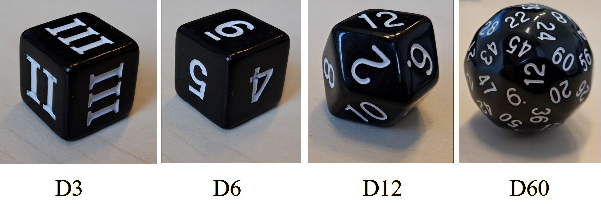
Inspired by an article on Ockham’s razor by Johnjoe McFadden, a previous post showed how a simple set of polyhedral dice can clarify the basic idea underlying Bayes factors. In the photo below, you see a family of four polyhedral dice: the D3, the D6 (this is the common six-sided die), the D12, and the D60.  

The Setup

You may assume each die is fair. I will first toss the D3 in order to select either the D6, the D12, or the D60. (if the D3 lands “I”, I will select the D6; if the D3 lands “II”, I will select the D12; and if the D3 lands “III”, I will select the D60).  Having selected one of the three die, I toss it and report to you only the outcome(s). It is your job to quantify and monitor the evidence, that is, the degree to which the data support the three rival hypotheses (i.e., D6, D12, or D60). 

Ockham’s Razor

Suppose the outcome is possible under each of the hypotheses. Let’s say we observe the outome “5”. Most people will intuit that this outcome provides evidence in favor of the D6. They may even be able to articulate why: the probability of seeing the outcome is 1/6 under the D6, but 1/12 under the D12, and 1/60 under the D60. The more sides a die has, the more thinly it has to distribute its predictions over the possible outcomes. In other words, D6 is rewarded for making precise, risky predictions that come true. This is exactly the principle that underlies the Bayes factor.

Jeffreys Already Did it

As McFadden acknowledges in his article, the idea that the Bayes factor is an automatic Ockham’s razor goes back to Harold Jeffreys’s work in the 1930s. In fact, in two of the three editions of Jeffreys’s book Scientific Inference (pp. 39-40 in the 1973 edition; pp. 37-38 in the 1957 edition), the scenario of the polyhedral die is discussed explicitly, albeit at a more abstract level.

Specifically, Jeffreys discusses the case of two rival hypotheses, which he labels q and ~q. The simple model q predicts the data to fall in a narrow interval ε (these are the predictions from the D6 die). The complex model ~q predicts the data to fall in a much wider interval E that encompasses ε (these are the predictions from the D60 die). Suppose the data fall inside the narrow interval ε (this is the fact that the outcome is “5”, a result that is consistent with both D6 and D60). Jeffreys then shows that the evidence (i.e., the Bayes factor) in favor of q over ~q equals E/ε. Jeffreys concludes:

Thus the more precise the inferences given by a law are, the more its probability is increased by a verification, even if the contradictory law also gives a prediction consistent with the observation. A single verification of a precise prediction may send up the probability of the law nearly to 1. (…)

We may say that to make predictions with great accuracy increases the probability that they will be found wrong, but in compensation they tell us much more if they are found right. (…) The best procedure, accordingly, is to state our laws as precisely as we can, while keeping a watch for any circumstances that may make it possible to test them more strictly than has been done hitherto. (Jeffreys, 1973, pp. 39-40)

This fragment is also cited in a recent paper where we outline a Bayesian perspective on severe testing (see also this blogpost).

References

van Dongen, N., Wagenmakers, E.-J., & Sprenger, J. (2023). A Bayesian perspective on severity: Risky predictions and specific hypotheses. Psychonomic Bulletin & Review, 30, 516-533.

Jeffreys, H. (1973). Scientific inference. Cambridge: Cambridge University Press.

McFadden, J. (2023). Razor sharp: The role of Occam’s razor in science. Annals of the New York Academy of Sciences, 1530, 8-17.