Abstract
Popular measures of reliability for a single-test administration include coefficient α, coefficient λ2, the greatest lower bound (glb), and coefficient ω. First, we show how these measures can be easily estimated within a Bayesian framework. Specifically, the posterior distribution for these measures can be obtained through Gibbs sampling – for coefficients α, λ2, and the glb one can sample the covariance matrix from an inverse Wishart distribution; for coefficient ω one samples the conditional posterior distributions from a single-factor CFA-model. Simulations show that – under relatively uninformative priors – the 95% Bayesian credible intervals are highly similar to the 95% frequentist bootstrap confidence intervals. In addition, the posterior distribution can be used to address practically relevant questions, such as “what is the probability that the reliability of this test is between .70 and .90?”, or, “how likely is it that the reliability of this test is higher than .80?”. In general, the use of a posterior distribution highlights the inherent uncertainty with respect to the estimation of reliability measures.
Overview
Reliability analysis aims to disentangle the amount of variance of a test score that is due to systematic influences (i.e., true-score variance) from the variance that is due to random influences (i.e., error-score variance; Lord & Novick, 1968).
When one estimates a parameter such as a reliability coefficient, the point estimate can be accompanied by an uncertainty interval. In the context of reliability analysis, substantive researchers almost always ignore uncertainty intervals and present only point estimates. This common practice disregards sampling error and the associated estimation uncertainty and should be seen as highly problematic. In this preprint, we show how the Bayesian credible interval can provide researchers with a flexible and straightforward method to quantify the uncertainty of point estimates in a reliability analysis.
Reliability Coefficients
Coefficient α, coefficient λ2, and the glb are based on classical test theory (CTT) and are lower bounds to reliability. To determine the error-score variance of a test, the coefficients estimate an upper bound for the error variances of the items. The estimators differ in the way they estimate this upper bound. The basis for the estimation is the covariance matrix Σ of multivariate observations. The CTT-coefficients estimate error-score variance from the variances of the items and true-score variance from the covariances of the items.
Coefficient ω is based on the single-factor model. Specifically, the single-factor model assumes that a common factor explains the covariances between the items (Spearman, 1904). Following CTT, the common factor variance replaces the true-score variance and the residual variances replace the error-score variance.
A straightforward way to obtain a posterior distribution of a CTT-coefficient is to estimate the posterior distribution of the covariance matrix and use it to calculate the estimate. Thus, we sample the posterior covariance matrices from an inverse Wishart distribution (Murphy, 2007; Padilla & Zhang, 2011).
For coefficient ω we sample from the conditional posterior distributions of the parameters in the single-factor model by means of a Gibbs sampling algorithm (Lee, 2007).
Simulation Results
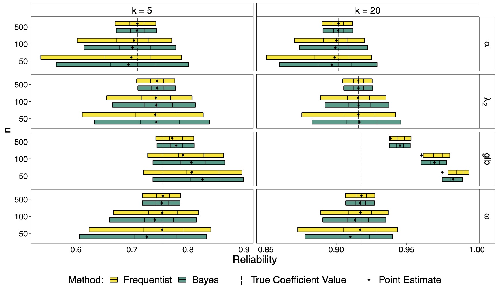
The results suggest that the Bayesian reliability coefficients perform equally well as the frequentist ones. The figure below depicts the simulation results for the condition with medium correlations among items. The endpoints of the bars are the average 95% uncertainty interval limits. The 25%- and 75%-quartiles are indicated with vertical line segments.
Example Data Set
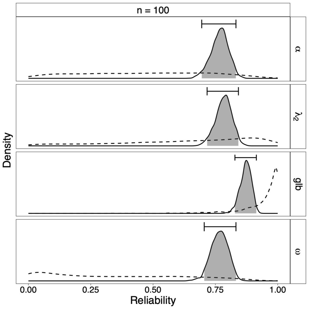
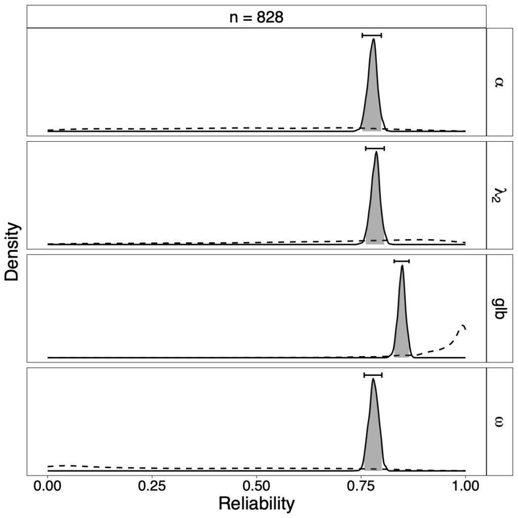
The below figures show the reliability results of an empirical data set from Cavalini (1992) with eight items and sample size of n = 828, and n = 100 randomly chosen observations. Depicted are posterior distributions of estimators with dotted prior densities and 95% credible interval bars. One can easily acknowledge the change in the uncertainty of reliability values when the sample size increases.
For example, from the posterior distribution of λ2 we can conclude that the specific credible interval contains 95% of the posterior mass. Since λ2 = .784, 95% HDI [.761, .806], we are 95% certain that λ2 lies between .761 and .806. Yet, how certain are we that the reliability is larger than .80? Using the posterior distribution of coefficient λ2, we can calculate the probability that it exceeds the cutoff of .80: p(λ2 > .80 | data) = .075.
Conclusion
The Bayesian reliability estimation adds an essential measure of uncertainty to simple point-estimated coefficients. Adequate credible intervals for single-test reliability estimates can be easily obtained applying the procedures described in the preprint, and as implemented in the R-package Bayesrel. Whereas the R-package addresses substantive researchers who have some experience in programming, we admit that it will probably not reach scientists whose software experiences are limited to graphical user interface programs such as SPSS. For this reason we have implemented the Bayesian reliability coefficients in the open-source statistical software JASP (JASP Team, 2020). Whereas we cannot stress the importance of reporting uncertainty enough, the question of the appropriateness of certain reliability measures cannot be answered by the Bayesian approach. No single reliability estimate can be generally recommended over all others. Nonetheless, practitioners are faced with the decision which reliability estimates to compute and report. Based on a single test administration the procedure should involve an assessment of dimensionality. Ideally, practitioners report multiple reliability coefficients with an accompanying measure of uncertainty, that is based on the posterior distribution.
References
About The Authors

